How can I combine the strengths of Python and imc FAMOS?
Both the imc FAMOS data analysis software and the Python programming language are very powerful and offer extensive functions for evaluating test & measurement data. These range from importing data from various file formats and graphical representation to automated calculations and report generation. Nevertheless, there are clear differences and limitations.
Compared to Python, imc FAMOS puts a focus on interactivity and usability in data analysis and plotting as well as the creation of own user interfaces for evaluations. Some of imc FAMOS' strengths lie in the following points:
- The interactive viewing of measurement data and comparisons of measurement series
- The interactive creation of meaningful plots
- Interactively analyzing measurement data, when it is not yet clear what you are looking for
- Performing engineering calculations without programming knowledge
- Automatically accounting for engineering units and sampling rates
- When creating your own user interfaces for semi-automated analysis
Python, on the other hand, scores with strengths like:
- Combination of measurement data analysis with other software functionalities
- Database, Data Lake, and Cloud Connectivity
- Choice of libraries for specialized mathematical calculations
- Platform independence
- Choice of example programs via the community
- Working with multi-dimensional and/or mixed-data-type lists
- Machine Learning
To get an impression of how imc FAMOS and Python can be used optimally, we will shed light on some details here and also show where the combination of imc FAMOS with Python offers advantages and what can be realized with it.
How does the display and review of measurement data work?
In principle, a distinction can be made between:
- Interactive plots
- Programmed plots based on templates
- Programmed plots without templates
In imc FAMOS, the primary way is interactive creation with the mouse. In most cases, the starting point is the QuickView window, which automatically displays all selected channels readily scaled and labelled. From there, various adjustments can be made:
- Using the mouse wheel, drag & drop, etc., you can zoom smoothly into the data to view individual areas in detail
- A measurement window dynamically shows the amplitudes at cursor positions and quantities such as RMS or the slope between them
- Drag and drop can be used to rearrange channels, change axes to dB scaling, or change the mode to a GPS plot or color map
- Labels, color overlays, line widths and other graphic elements can be adjusted via configuration dialogs, similar to Microsoft Excel
- Markings of peak values, intervals between events or the like can be created with the mouse
Creating a display using programming, but based on a template is possible by saving the interactively created window as a configuration file (CCV) and loading it later. The code for this is e.g.:
CwLoadCCV("Curve6335", "Speed_Engine_RPM.ccv")
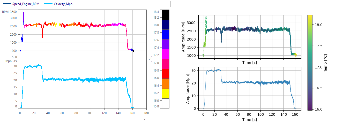
A programmed representation without a template requires a number lines of code in imc FAMOS as well as in Python:
;--- Display ---
CwNewWindow("Curve6335","show")
 CwDisplaySet("grid",1)
 CwDisplaySet("color palette",1)

;--- Channels ---
CwNewChannel("append new axis",Speed_Engine_RPM)
CwNewChannel("append last axis",Ambient_Temp)
CwNewChannel("append new cosys",Velocity_Mph)

;--- RPM display: Set order of magnitude and color overlay ---
CwSelectByIndex("cosys",1)
 CwSelectByIndex("y-axis in cosys",1)
  CwAxisSet("exponent",0) ; set order of magnitude to 0 so we see 3000 RPM instead of 3*10³ RPM
  CwSelectByIndex("line in axis",2) ; ambient temperature line
   CwSelectByIndex("data in line",1)
    CwDataSet("function",1) ; activate color overlay

;--- Increase line width ---
for i = 1 to 2
   CwSelectByIndex("cosys",i)
    CwSelectByIndex("y-axis in cosys",1)
     CwSelectByIndex("line in axis",1)
      CwLineSet("width.screen",0.53)
end
fig,axs = plt.subplots(2,sharex='all')

# First Plot with Colorbar
axs[0].plot(x,y1,lw=0.3,alpha=0.3,c='k') # Thin black line
sc = axs[0].scatter(x,y1,c=c1,s=2,alpha=0.9) # Colored scatter
cbar = fig.colorbar(sc, ax=axs.ravel().tolist()) # Make colorbar for all axes
cbar.set_label('Temp ['+c1_label+']')

# Second Plot
axs[1].plot(x,y2,lw=0.5,alpha=0.9)

# Adjust Axes
for ax in axs:
    ax.set_xlabel('Time ['+x_label+']')
    ax.grid()
axs[0].set_ylabel('Amplitude ['+y1_label+']')
axs[1].set_ylabel('Amplitude ['+y2_label+']')
plt.show()
How about calculations?
Simple formulas can be typed in a similar and quite simple way in both imc FAMOS and Python. For example, the calculation of the root of 2 is done with:
a = sqrt(2)
import math
a = math.sqrt(2)
print(a)
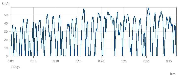
The calculation of how long a public bus has been at stops in total, based on its speed signal, can be expressed in this way:
imc FAMOS (with automatic use of sampling rate):
speed0 = speed < 0.5
speed0totaltime = sum(speed0) * xdel?(speed0)
Python (for simplicity with fixed coding of sampling rate):
speed0 = speed < 0.5

speed0totaltime = sum(speed0) * 0.05
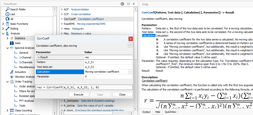
For more complex functions, imc FAMOS displays a wizard and a help text with examples. Python does not offer such integrated assistance, but refers to an extensive online documentation and user forums for understanding the functions.
How are units taken into account?
Units as well as time stamps are firmly linked to the data in imc FAMOS. Therefore, they also appear automatically when opening curve windows. They can be explicitly set by functions, but also imported directly with the data files, implicitly specified in formulas and are also automatically converted with calculations:
P = 230 'V' * 3 'A' ; Unit for P is automatically 'W'
SetUnit(speed, "km/h", 1)
ConvertUnit(speed, "m/s", 1) ; Conversion to m/s
Similar to how in this example the unit automatically becomes Watts, conversions also take place for integrals, PSD calculations, etc. The ConvertUnit function enables error-free conversion of data into specific target units, optionally forcing NIST rules. If a conversion is not possible, the whole analysis sequence fails instead of continuing to calculate with incorrect values, which is the risk with manual conversions.
In this way, the units consistently contribute to plausibility checks and rapid understanding of the data.
In Python, units are usually set manually, or carried along with the data with the help of dictionaries or lists. There are different approaches and some tools such as UnitPy, but no standardized ways. The programmer is therefore responsible for consistent units himself.
Is it possible to create sub-functions?
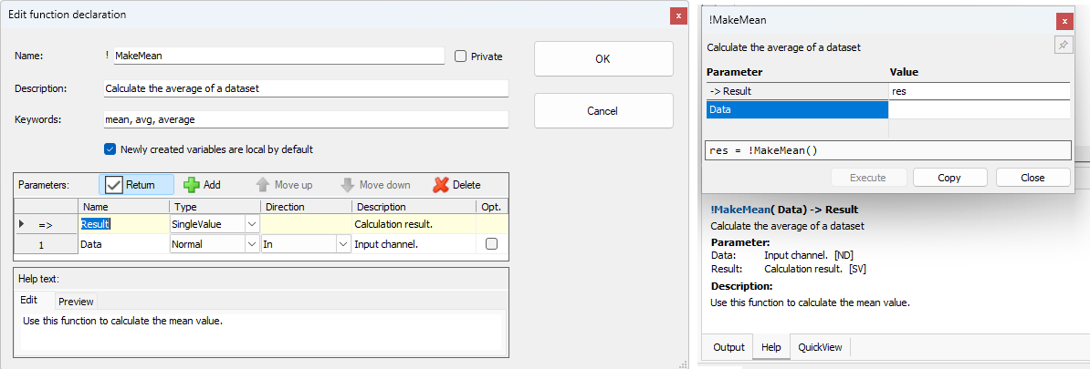
Sub-functions are possible in both solutions. In imc FAMOS, they are called sequence functions and are created using a wizard. Input parameters, return value and description texts are defined there. Later, just as with the inbuilt functions, an assistant is offered for use and the help texts are displayed.
The content of the sequence function in the example would be:
Result = mean(Data)m = !MakeMean([1,2,3,4])In Python, both creation and content are implemented through source code, e.g.:
import numpy as np
def makemean(data):
    # Calculate the average of a dataset.
    # Use this function to calculate the
    # data: Input channel.
    # Returns the calculation result. Single value.
    # Tags: mean, avg, average
    value = np.mean(data)
    return value

m = makemean(np.array([1,2,3,4]))
Can I automate creation of Office documents?
This is possible in imc FAMOS as well as in Python, but imc FAMOS specializes in PowerPoint and Excel remote control. Generating a PPTX report can be done with the following commands, for example:
PptOpenPresentation("c:\temp\template.pptx", 0)

PptAddSlides(1, "c:\temp\plotpagetemplate.pptx")
PptSetText(1, "Heading", "Example report")
CwSelectWindow("ForceVsDisplacement")
PptSetCurve(1, "plot1", 1, 0, "printer")

PptSavePresentation("c:\temp\report.pptx")
PptClosePresentation()
Generating a Word report with Python looks very similar:
from docx import Document
# If docx missing, run in terminal: pip install PyDocX

doc = Document('c:\\temp\\template.docx')

doc.add_page_break()
doc.add_heading('Example report')
doc.add_paragraph('Example plot')
doc.add_picture('c:\\temp\\plot1.png')

doc.save('c:\\temp\\report.docx')
In what ways can imc FAMOS combine with Python?
Sequences in imc FAMOS can be mixed with Python code. There are the following options:
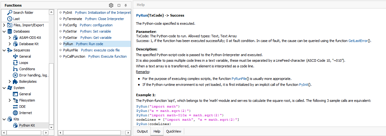
- Calling a set of Python commands with PyRun()
- Calling an explicit Python function with PyCallFunction
- Calling a .py file with PyRunFile() if you develop the file externally, e.g. with Visual Studio Code
For example, the following sequence can compute a square root using Python:
PyRun("import math")
result = PyCallFunction("math", "sqrt", 2)
Even complex functions such as a discrete wavelet transformation can be achieved with it:
PyRun(["import pywt", "import numpy as np"])
result = PyCallFunction("pywt", "cwt", signal, !CreateSignal.Ramp(1, 129, 1, 129), "gaus1")
If a function such as cwt returns two results, a group of two variables is created by imc FAMOS. For calling a complex script (or an external source code file), variables can also be explicitly passed to the Python environment, and the results transferred back. This way, exchanging variables can be realized generically and dynamically.
For example, the following is how to load two channels from an Apache Parquet file:
PySetVar("", "p", "c:\temp\weather.parquet")

PyRun([
"import pandas as pd",
"df = pd.read_parquet(p)",
"MinTemp = df['MinTemp'].to_numpy()",
"MaxTemp = df['MaxTemp'].to_numpy()"])

MinTemp = PyGetVar("", "MinTemp")
MaxTemp = PyGetVar("", "MaxTemp")
Stretching a FAMOS call over multiple lines, as seen here, can be achieved by using Shift+Enter and is recommended for short Python scripts.
Reading a python-typical pkl file is very similar, for example:
PyRun([
"import pickle",
"with open('c:\\temp\\famos.pkl', 'rb') as fp:",
"    famosdata = pickle.load(fp)",
"values = famosdata['value_y']"])

values = PyGetVar("", "values")
The exchange between imc FAMOS and Python takes place directly in the PC's RAM and is therefore high-performance and fast even for large amounts of data.
Typical use cases for this combination are, on the one hand, the extension of FAMOS by:
- Specialized calculation algorithms such as power quality analysis for wind turbines according to IEC 61400, wavelet transformation or the generation of red noise (1/f² noise)
- Cloud or web service connection to retrieve or upload data or analysis results
- Specialized database connection
- Import data from specialized file formats, e.g. parquet, json or pickle files
- Complex processes that can be implemented more efficiently in a universal programming language
On the other hand, this combination also offers the possibility to extend Python programs, for example to:
- Create your own user interfaces for semi-automated analysis
- Perform an interactive data review and analysis if the Python evaluation program produces unexpected results
- Interactively select measurements or channels before starting the analysis
What examples and assistance exist for the Python integration in imc FAMOS?
The best way to get started is often the wizard for running a Python script. Its purpose is to generate a FAMOS sequence function around a Python script. It gradually asks you to enter all relevant information:
- Name and description of the sequence function
- The Python code or an external Python script file
- The list of variables that the script will process and the number of results it will return
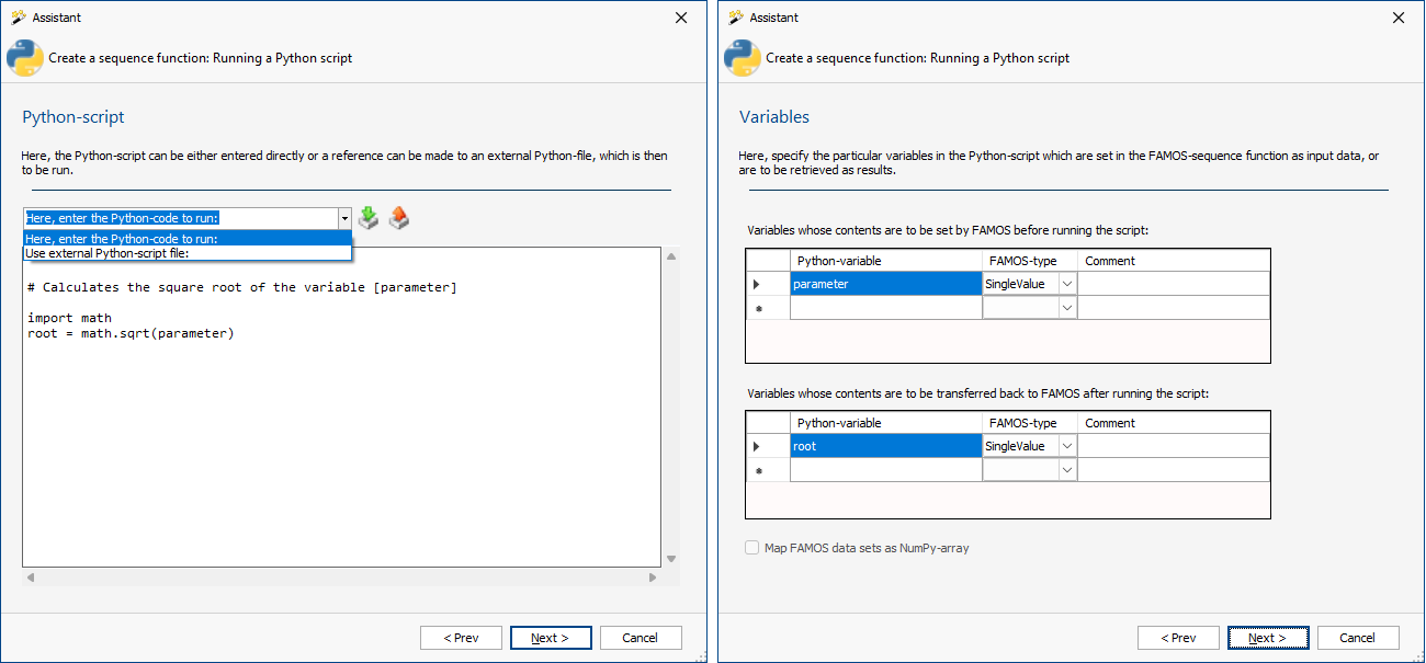
At the end, the resulting sequence function can be tested before it is generated as a file. All fields are pre-assigned in such a way that a meaningful example is created even without input (Calculating a square root, the function is then called e.g. "!PythonLib.CalcSquareRoot"). A call is then made with, for example:
a = !PythonLib.CalcSquareRoot(2)
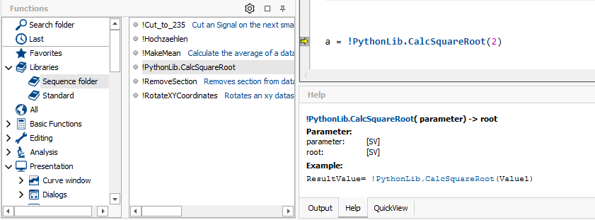
The function also automatically comes with an assistant for selecting the parameters as well as a help text that is automatically displayed.
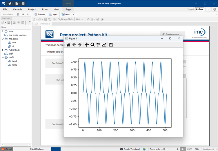
In addition to this wizard, a demo project "Python" is available, which is also always part of the imc FAMOS installation. It showcases examples of how histogram, percentile or FFT calculations can be performed with Python code and also contains sample measurement data so that it can be used directly and adapted to one's own purposes.
Finally, it is also possible to get started via the individual functions, which are summarized in the category "Python Kit". These eight functions also each have description texts with examples, on the basis of which you can easily create your own solution.
Conclusion
For many situations in which measurement data has to be evaluated, imc FAMOS offers everything you need:
- Import of data from many file formats
- Quick and easy plotting of measurement data
- Quick comparison of measurement series
- Easy creation of meaningful plots including markers
- Extensive engineering calculations that can be applied interactively without programming knowledge
- High performance in display and calculations
- Interactive creation of reports and custom user interfaces for semi-automated analysis
- Creation of fully automated analyses including the generation of PowerPoint files or similar.
Many of these aspects can be realized with Python too, but a bit more cumbersome there. Python programmers who want to achieve more interactivity in data viewing and processing can therefore use imc FAMOS for this purpose and call up their existing analysis scripts where suitable.
Since imc FAMOS is limited in some other aspects in order to remain manageable by measurement engineers without much programming knowledge, it also reaches its limits in some cases.
In these cases, the interface to Python makes it possible to extend imc FAMOS in practically unlimited ways and to fully exploit the strengths of both packages.
The trial version of imc FAMOS includes a demo project with which this extensibility can be tried out as desired.
FAQ
Which Python versions are supported by imc FAMOS?
In version 2026 R1, imc FAMOS supports Python versions 3.8 to 3.14 and NumPy versions 1.19 bis 2.3 Future versions will support later versions as well.
The call to my Python file fails because Pandas was not found, but it is installed. What's the problem?
Possibly, the package is only installed locally for the user. Please check with "pip list --user" if this is the case. If so, please reinstall it for all users.
I'm using Anaconda, and the Python call from imc FAMOS doesn't work. What can be the problem?
In many cases, everything works smoothly with an Anaconda environment. If this is not the case for you, please try to start imc FAMOS from an Anaconda terminal window (cmd.exe or Powershell prompt).
In addition to the values of a channel, can I also transfer its properties, e.g. unit and sample rate, to Python?
Yes, although it has to be created individually, as there is no universal concept for it on the Python side. For example, it has proven to be a good idea to create a Group on the FAMOS side that contains the properties as single-value variables in addition to the channel itself. This Group can be transferred to Python as a whole and then becomes a Dictionary there.
How can I integrate a particular Python environment or use it for execution?
Currently, imc FAMOS does not offer direct support for environments. However, one control option is to add the corresponding path with the Python command sys.path.insert directly after PyInit. The index 0 is important. For example, if the environment path is c:\py_venv, the call is:
PyRun("sys.path.insert(0, 'c:\py_venv\lib\site-packages')")
How can I access the FAMOS working directory in the Python script?
In imc FAMOS there is no global working directory, so it is recommended to pass target directories as text variables to the Python script.
My PyPlot grows with repeated script calls instead of always being structured in the same way. What am I doing wrong?
Please close the plot with plt.close() at the end of the script if you don't need it anymore. It does not automatically close after execution.
How do I find out which console outputs my Python script has created with print after I have called it from FAMOS?
All print outputs are displayed in the imc FAMOS output window. If the Python script fails due to an error, the error details are displayed there instead.